CS 205 Final Project
Parallelizing an ILP Assignment Problem
Results
Setup
We modeled the underlying ILP with pulp using the GNU GLPK as the back-end solver. We used mpi4py to parallelize solution finding.
Notation
Let $m$ denote the number of students and $n$ denote the number of classes. Let $x_{ij}$ be a binary variable with $x_{ij} = 1$ indicating that student $i$ is assigned to class $j$, for $i = 1, ..., m$, $j = 1, ..., n$.
Objective function
Our true goal in the ILP is not to find the "best" ILP solution — we actually evaluate solution fitness in the non-linear step — instead we are simply trying to generate as many feasible solutions as possible subject to our hard constraints. We create an arbitrary objective function:
$$\operatorname{min} Z = \sum_{j=1}^{n} \sum_{i=1}^{m} x_{ij} \cdot i \cdot j$$
This objective function can be used to get the solver to generate a different feasible solutions. Specifically, we can take the objective function minimum found in the last iteration — call it $z_{t-1}$ — and add a new constraint for the current iteration that the objective function $Z > z_{t-1}$. For our data set, our solver found a minimum value for the objective function of 9,227 and a maximum value of 11,534. Thus, the upper bound on the number of solutions we could generate is 1,608. However, the solver is not always able to find a solution at each integer within this range. This is especially true near the endpoints of the domain (we were able to find a total of 1,409 solutions for our dataset). Thus, we face two issues when trying to parallelize this process: first that the ILP solver takes different amounts of time for each solution (ranging from about one second to one minute), thus creating imbalanced workloads, and secondly that we don't know ahead of time how many times the solver will be called within a given range.
Note: some solvers are able to generate additional feasible solutions from the same LP model, but many are not. Though we opted to use GLPK for benchmarking purposes, we wanted to avoid making assumptions about the solver. For that reason, we chose this method of an artificial objective function with iterative constraints in order to generate multiple feasible solutions.
Constraints
- All decision variables must be binary.
$$x_{ij} \in \{0, 1\}, \; \forall \; i \in \{1, ..., m\} \text{; } j \in \{1, ..., n\}$$
- Every student must be assigned to a class.
$$\sum_{j=1}^{n} x_{ij} = 1, \; i \in \{1, ..., m\}$$
- A maximum class size $k$ must be respected.
$$\sum_{i=1}^{m} x_{ij} \leq k, \; j \in \{1, ..., n\}$$
- Every student must be in a class with one of his or her designated friends (in a friend list $L_i$ of friends for student $i$).
$$x_{ij} \leq \sum_{s \in L_i} x_{sj}, \; i \in \{1, ..., m\} \text{; } j \in \{1, ..., n\}$$
- Certain other constraints involving the male/female ratio in a class, or students who should be kept apart.
Basic implementation
The simplest implementation using MPI is to start each process off with a roughly equal portion of the integers in between the absolute min and max of the artificial objective function, and let them simply work through their respective assignments without communicating further until work collection by the root process.
The obvious problem with this method — we'll call it the "naive" implementation — is that some processors may finish long before the others and waste time doing nothing. Nonetheless, there is a significant initial speedup achieved simply by dividing up the work among many processors. We seek to improve on this initial improvement by being smarter about keeping all processes employed.

Distributed load balancing
One way to split up work in MPI is to start each process off with a roughly equal portion of the domain (as in the naive implementation), but let them communicate directly with one another if they run out of work. In order to do this, each process runs with a work thread that solves the ILPs and a communication thread that sends out requests for work when the work thread finishes and also "listens" for requests from other processors. When a processor receives a request for work, if it has more than a minimum threshold of work left within its given range, it hands off half of the work to the requesting processor. If it does not have work, then it sends a rejection and the processor requesting work will then move on to request work from the next processor. If the processor receives enough rejections, then it simply gives up and terminates (although it's communication thread will stay alive until the all processors are done in order to send out rejections when it receives work requests).
The major problem with this method is that having each processor running multiple threads slows down the speed at which they do work. To alleviate this issue, we have the communication thread pause for two seconds between each iteration of its loop. This works well for a low number of processors, but does not scale well since the communication overhead increases with the number of processors, so the communication thread does a significant amount of work despite the pauses (we experimented with various pause lengths, but increasing the pause length too much slows down the average response time when processors request work. We found 2 seconds to be a good balance). Additionally, even without any pause, as the number of processors increases, so too does the response time since each processor must check for messages from all other processors.
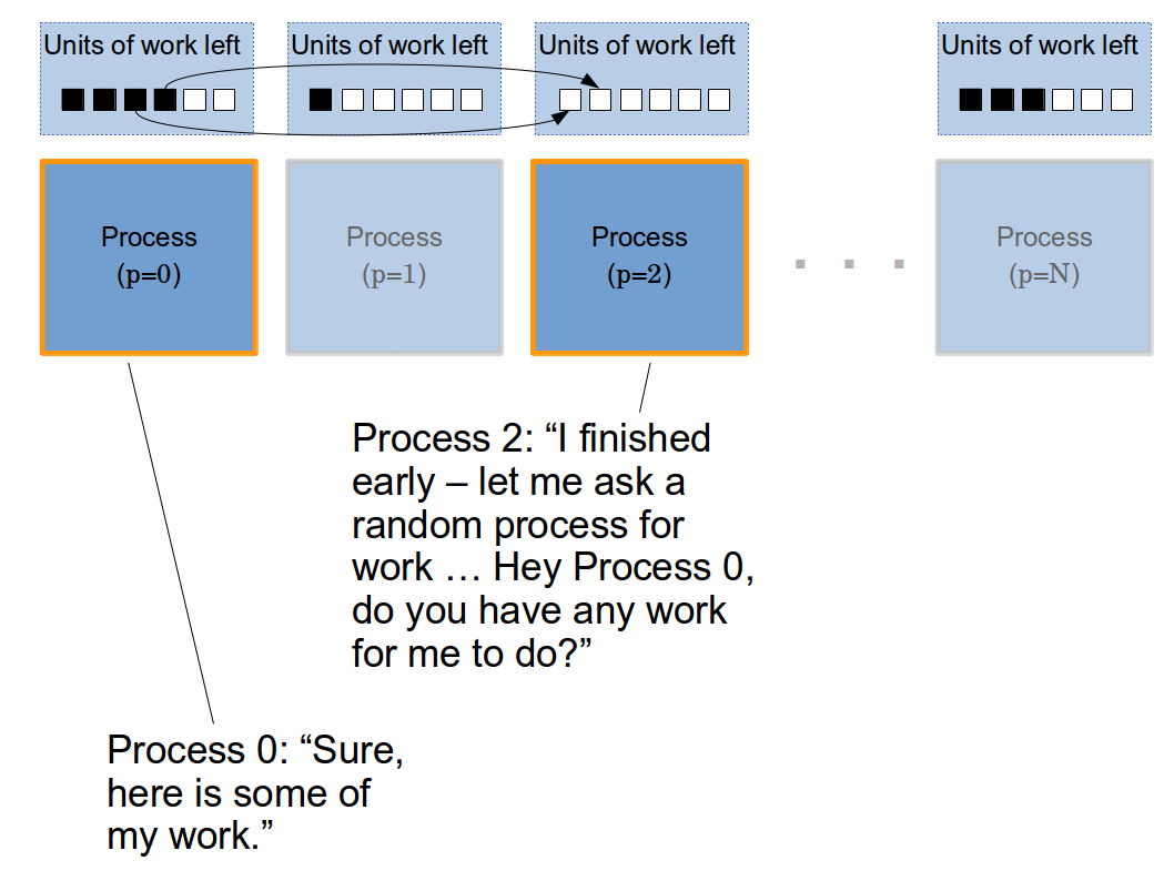

As the results above show, with fewer processors, this was a relatively fast and efficient method. However, the communication overhead increases quickly as the number of processes is increased, which actually causes the process to slow down when too many processors are used. Another reason that it doesn't scale well for this problem is that we have a limited domain. When using 256 processors, each processor gets a "chunk" of about 6 integers from the range between 9,927 and 11,534. With such a small amount of work to be completed and a large amount of communication overhead slowing down each processor, it is more efficient to simply divide the work up "naively" and process it without any communication. Because of these scaling issues, we decided to implement the master/slave implementations discussed below.
| processors | load balancing | time (s) | speedup | efficiency |
|---|---|---|---|---|
| 1 | --- | 13500.3095 | --- | --- |
| 2 | No | 7150.7547 | 1.89 | 0.94 |
| 4 | No | 3910.5397 | 3.45 | 0.86 |
| 8 | No | 2411.4662 | 5.60 | 0.70 |
| 16 | No | 1096.7792 | 12.31 | 0.77 |
| 32 | No | 650.0861 | 20.76 | 0.65 |
| 64 | No | 381.0861 | 35.43 | 0.55 |
| 128 | No | 221.8088 | 60.86 | 0.48 |
| 256 | No | 143.8961 | 93.82 | 0.37 |
| 2 | Yes | 6799.1015 | 1.99 | 0.99 |
| 4 | Yes | 3641.5851 | 3.71 | 0.93 |
| 8 | Yes | 1787.092 | 7.55 | 0.94 |
| 16 | Yes | 1063.6516 | 12.69 | 0.79 |
| 32 | Yes | 555.0021 | 24.32 | 0.76 |
| 64 | Yes | 401.2980 | 33.6416 | 0.49 |
| 128 | Yes | 217.4343 | 62.09 | 0.49 |
| 256 | Yes | 542.4713 | 24.89 | 0.10 |
Master/slave model
In the first iteration of master/slave, each process initially gets an even chunk of the integers in between the absolute min and max of the artificial objective function. Like the naive implementation, we do not yet do any load balancing. Additionally, we have one fewer process than the naive version because the master does not yet do any work. Although it seems probable that load balancing will have a net positive impact, we first would like to observe performance without doing so — this way we can quantify the benefits of load balancing, and see if the added overhead is worthwhile.
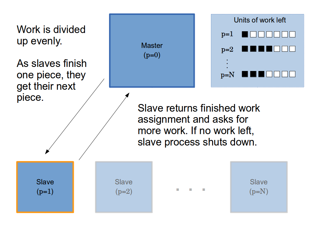
Like the naive implementation, this method resulted in excellent speedups over the serial version — the following graph shows both speedup and efficiency with different numbers of processors.

Master/slave model with load balancing
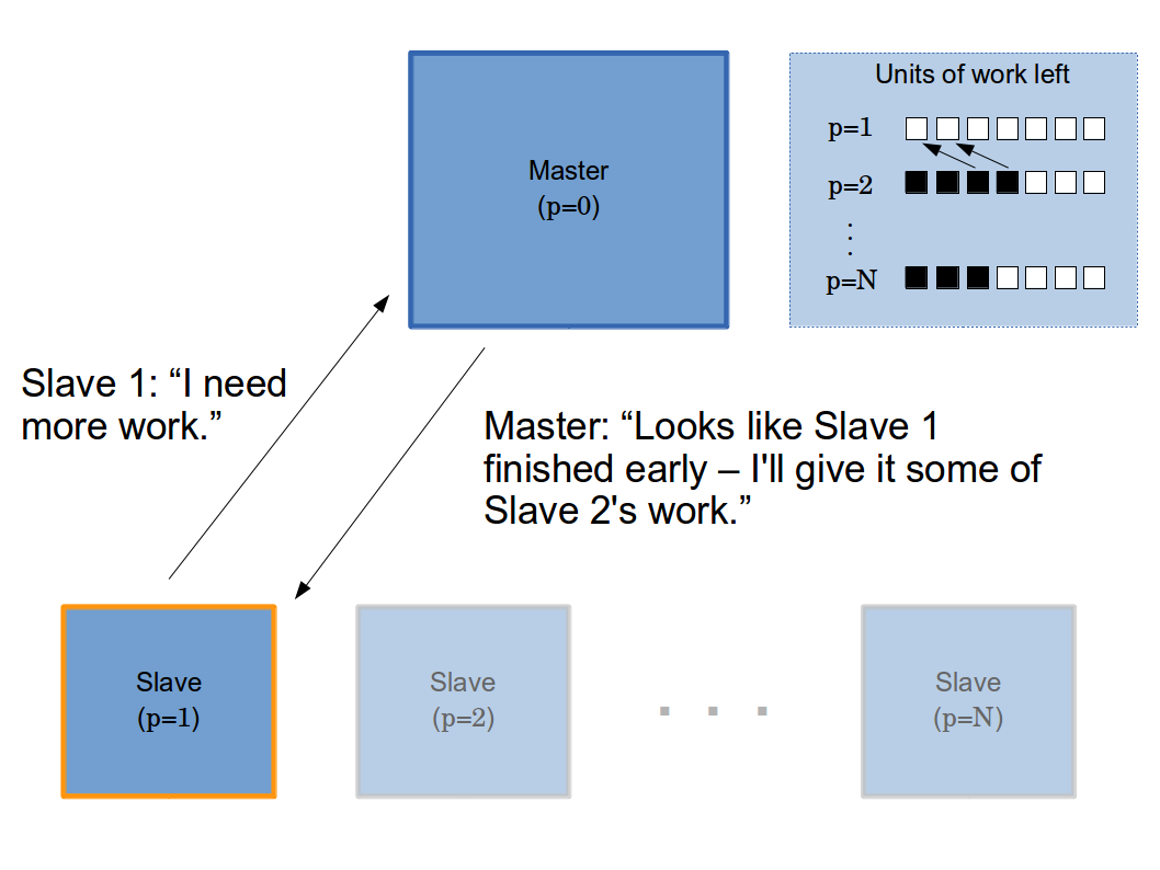
To be even more efficient, we don't want any of our slave processes to finish early (which they often do because feasible solutions are not evenly distributed through the space of integers being divided up). In our next iteration, we implemented a scheme where the master would attempt to redistribute work from the slowest process to any process that had finished all of its initial work assignment.

| processors | load balancing | time (s) | speedup | efficiency |
|---|---|---|---|---|
| 1 | --- | 13500.3095 | --- | --- |
| 4 | No | 4922.5975 | 2.74 | 0.69 |
| 8 | No | 2212.6460 | 6.10 | 0.76 |
| 16 | No | 1148.0969 | 11.76 | 0.73 |
| 32 | No | 581.3491 | 23.22 | 0.73 |
| 64 | No | 325.5046 | 41.48 | 0.69 |
| 128 | No | 186.2928 | 72.49 | 0.57 |
| 256 | No | 161.1719 | 83.76 | 0.33 |
| 4 | Yes | 4538.3395 | 2.97 | 0.74 |
| 8 | Yes | 1965.5124 | 6.87 | 0.86 |
| 16 | Yes | 961.8448 | 14.04 | 0.88 |
| 32 | Yes | 481.9911 | 28.01 | 0.88 |
| 64 | Yes | 300.3186 | 44.95 | 0.70 |
| 128 | Yes | 179.7172 | 75.12 | 0.59 |
| 256 | Yes | 130.6939 | 103.30 | 0.40 |
Using MapReduce to generate even more solutions
The ultimate goal was to get high fitness scores from the non-linear heuristic. To be even more exhaustive, we took all feasible solutions from the parallelized ILP. These solutions were fed into a MapReduce program which perturbed each arrangement by switching every possible pair of students and then checking the non-linear fitness of the perturbed solution. We wrote this MapReduce job in Python using the mrjob package, and ran it on 10 m1.large Amazon AWS EC2 instances.
While these perturbed solutions were not guaranteed to obey the hard constraints — many did not — that did not necessarily mean they would all have worse fitness scores (although it was likely since the heuristic heavily penalizes violated constraints). We wanted to get an idea of how sparse higher fitness scores would be for solutions that were "near" those generated by the ILP.
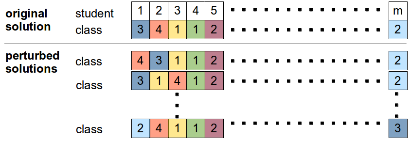
As expected, it turned out that very few of the generated perturbations had fitness scores that were higher, and of those that did the difference was small. Of over 6,000,000 perturbed solutions evaluated:
- Only 7,718 did not have worse fitness scores than the original solution.
- Of those 7,718, only 772 scored higher than the original.
- Of those 772 that scored higher, the largest observed difference between the original fitness score and the perturbed solution score was only 500 points — not a significant difference for scores that are routinely in the neighborhood of 17,000. In fact, most differences were fewer than 200 points.

Conclusion
We achieved a gratifying speed increase — over 100x — by parallelizing this problem, going from the order of almost 4 hours to about 2 minutes using 256 processors. Even the most naive implementation represented a massive improvement simply by moving from serial to parallel.
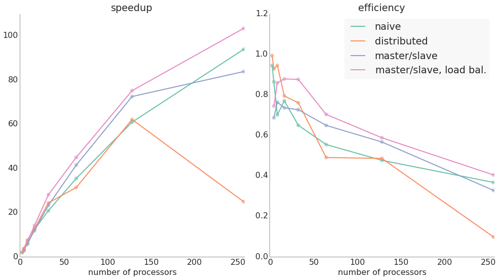
With large numbers of processors at your disposal, the master/slave model with load rebalancing is the most efficient of our methods. If the domain was significantly larger such that there were many more solutions to be found, we believe that you could even potentially implement a model with two or more masters and many slaves that might run more efficiently with very large numbers of processors. But we did not implement this since we did not think that we would see speedups for a domain of our problem's size (not to mention that for practical purposes, we did not have access to a cluster where we could easily test our implementations on more than 256 processors!). In practice, if this model is used for actual class placements, it will probably be run on a laptop or desktop computer with 2-8 cores. In that case, the most sensible implementation to use would be the distributed load balancing one, since that is more efficient with smaller numbers of processes, even though it does not scale up well.
When using this model for actual class placements, the school is likely to want the results from the top 4 or 5 placements as scored by the non-linear evaulation function. Integrating the code with the software that the school currently uses to place students was outside the scope of this project. However, due to the significant speedups from utilizing multiple cores, especially for low numbers of cores where efficiency is high, it is likely that parts of this project will be implemented into the school's software in the future.
Insights, possible improvements and other musings about the project
In working on this project, we learned quite a bit about MPI. There were an unknown number of solutions within the search domain, so figuring out how to split it up required quite a bit of trial and error. For example, we found that if we didn't set a minimum threshold for how much work processors could hand off to each other, it often led to repeated work being done since feasible solutions were not distributed evenly along the domain.
In the distributed load balancing implentation, we had to come up with an implementation that allows processors to communicate with each other while also doing their own work. To accomplish this, after much frustration, we eventually found that we could use threading. However, threading added a whole new dimension to the complexity of the program, since we had to keep track of not only different processors, but also different threads on each of those processors. Implementing this was challenging, but rewarding as well.
Originally, we also intended to create an implementation where each processor broadcasts its current workload to every other processor after each step. However, after much effort, we ultimately abandoned this approach. Looking at similar projects online, it seems that mpi4py does seem to offer a non-blocking broadcast function (Ibcast) that might have helped. Unfortunately, this function is not mentioned in the official documentation and we were also told that it is not very reliable, so we did not try to use it. In any case, this implementation probably would have had considerable communication overhead and so would not have given us any speedups over our other implementations.
As mentioned in the conclusions above, it also would have been interesting to implement a master/slave model with multiple masters that communicate with each other, but given our data set and general approach, we don't think that this would have given us significant speedups, although it would be interesting to try on a larger ILP problem with more solutions to iterate through.
Using integer linear programming was just one method of solving this type of problem. There are others, such as stochastic local search tecniques that could be parellelized; doing so would be an interesting followup to this project.